Technically this could be any transforming of a variable or multiple variables so it could include dichotomising a continuous variable into (say) high/low or standardising where the aim is to make a lot of different variables all have the same mean and standard deviation. However, it is generally used for transformations that bring a variable into a distribution shape more like a Gaussian distribution in order to make it fit the assumptions of a parametric test involving the variable.
With the increasing shift away from null hypothesis tests and the increasing use of bootstrapping to avoid assuming that things come from Gaussian distributions, I think transformations are getting pretty rare now in the MH/therapy research world but here are the gory details just in case you hit a report using them but not really explaining them.
Details #
Here’s an example. Imagine you have 710 values from some measure. Here are the raw data (in a histogram with a smoothed density curve on top).
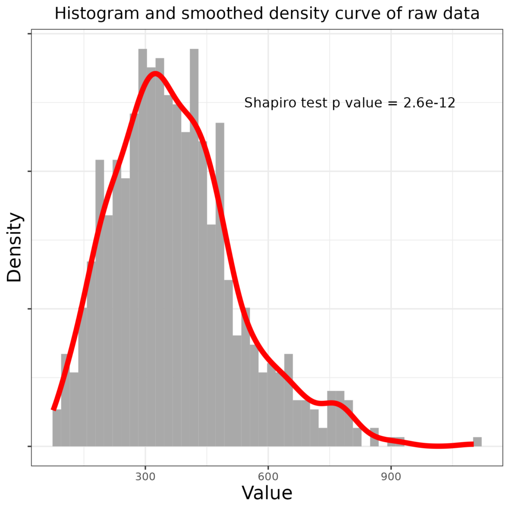
We can see that the distribution is “right skew”: it has a “tail” off to the right. The Shapiro-Wilk test (q.v.) is highly statistically significant showing that it’s vanishingly unlikely that this quite large sample arose from sampling from a population in which the values have a Gaussian distribution.
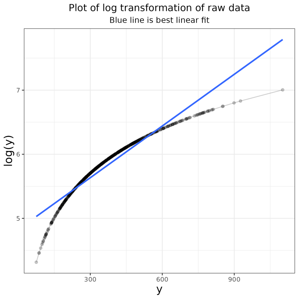
In this situation, before bootstrapping (q.v.) rendered the preoccupation with Gaussian distributions and parametric versus non-parametric tests less important, a researcher might have tried to find a transformation of the data that pulled them closer to a Gaussian distribution. She might have tried taking the log of the values (as logs shrink large numbers much more than they shrink small numbers so they reduce right skew). Here’s that log (to base e) transform of the raw data. I have added a best fit linear regression line in blue to emphasise that the transformation has reduced the higher values and increased the smaller values relative what a linear transform would have done.
How has that affected the distribution?
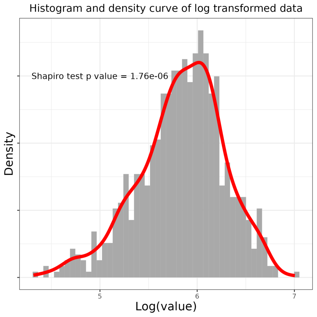
That has overdone it and now the distribution is slightly left skew and though the misfit according to the Shapiro-Wilk test has been reduced, this is still not nearly Gaussian. What about using a square root transformation (square roots, only, for our purposes applicable to positive numbers, also reduce large numbers more than smaller ones). Here is the transformation mapping this time mapping the square root transform rather than the log transform.
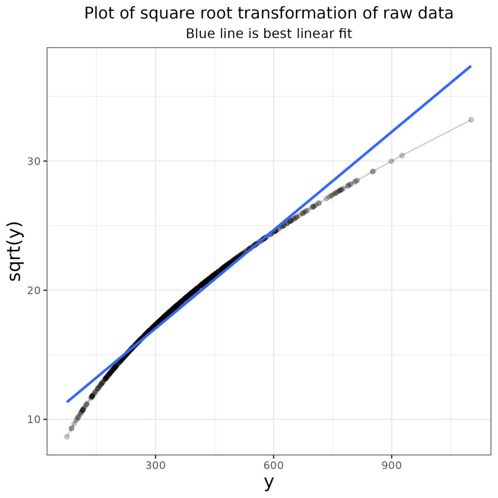
You can see that that has again, relatively, shrunk the larger values and increased teh smaller values but less so than the log transform did. So how has that changed the distribution?
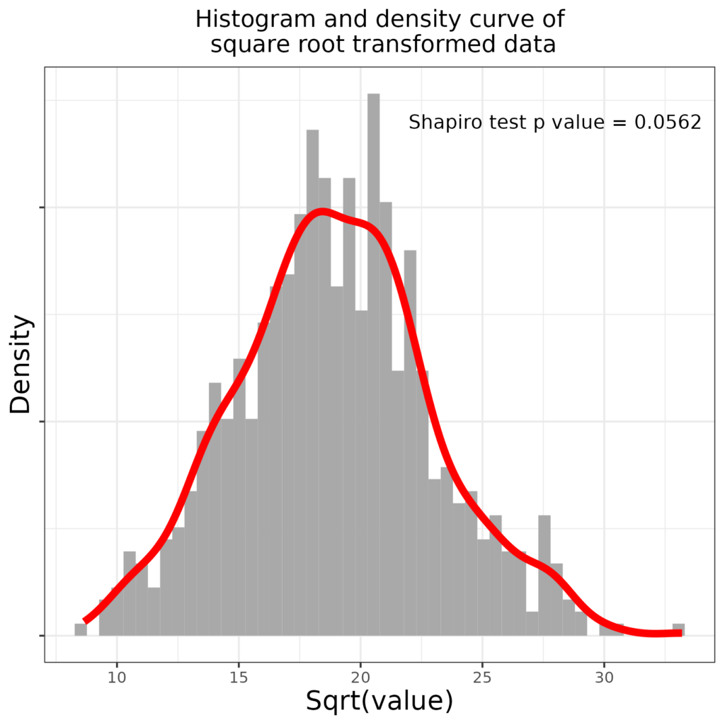
Bingo! The distribution is now, very narrowly, not statistically significantly implausible to have arisen by sampling from a Gaussian population as the Shapiro-Wilk test p value is .0562, above the conventional “< .05” criterion.
Try also #
Bootstrapping
Dichotomising
Distribution shape
Gaussian distribution
Null hypothesis testing (NHST)
Parametric tests
Shapiro-Wilk test
Skewness
Standardising/normalising
Chapters #
A bit esoteric these days, not covered in the book.
Online resources #
None yet, low on my priorities!
Dates #
First created 1.iii.24, tweaked links 21.vi.24.

